Introduction
What is RL? A short recap
In RL, we build an agent that can make smart decisions. For instance, an agent that learns to play a video game. Or a trading agent that learns to maximize its benefits by deciding on what stocks to buy and when to sell.
To make intelligent decisions, our agent will learn from the environment by interacting with it through trial and error and receiving rewards (positive or negative) as unique feedback.
Its goal is to maximize its expected cumulative reward (because of the reward hypothesis).
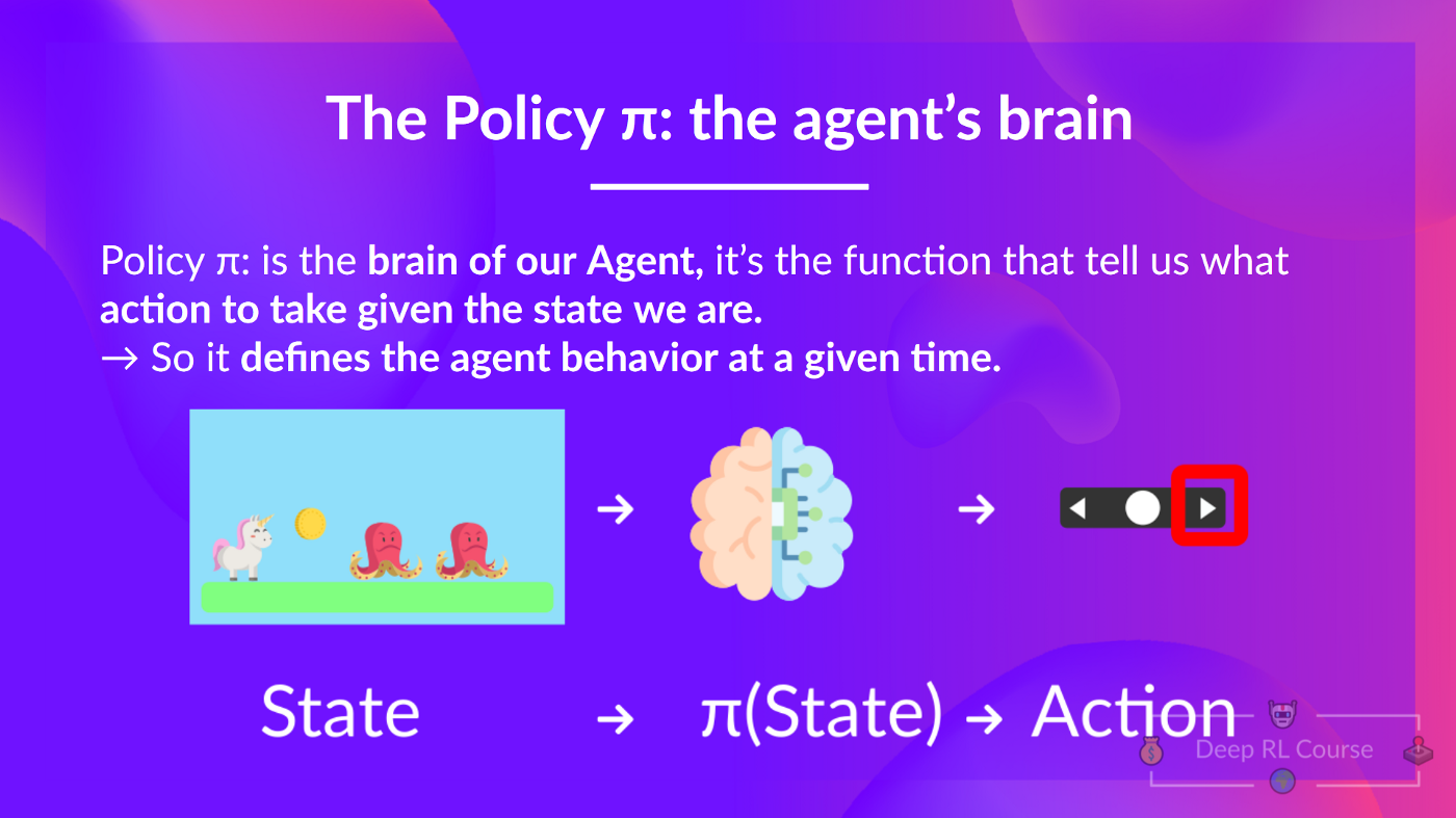
The agent’s decision-making process is called the policy π: given a state, a policy will output an action or a probability distribution over actions. That is, given an observation of the environment, a policy will provide an action (or multiple probabilities for each action) that the agent should take.
Our goal is to find an optimal policy π* , aka., a policy that leads to the best expected cumulative reward.
And to find this optimal policy (hence solving the RL problem), there are two main types of RL methods:
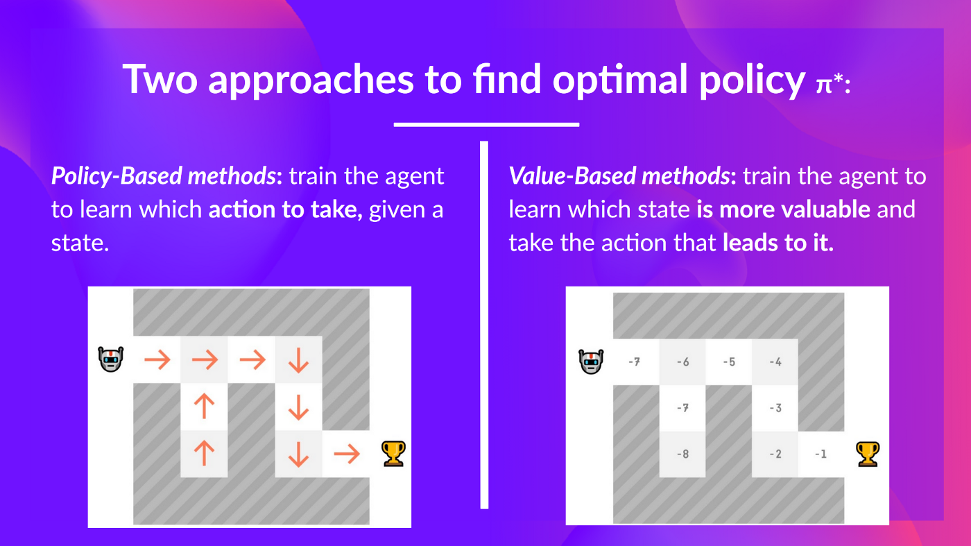
- Policy-based methods: Train the policy directly to learn which action to take given a state.
- Value-based methods: Train a value function to learn which state is more valuable and use this value function to take the action that leads to it.
Two types of value-based methods
In value-based methods, we learn a value function that maps a state to the expected value of being at that state.
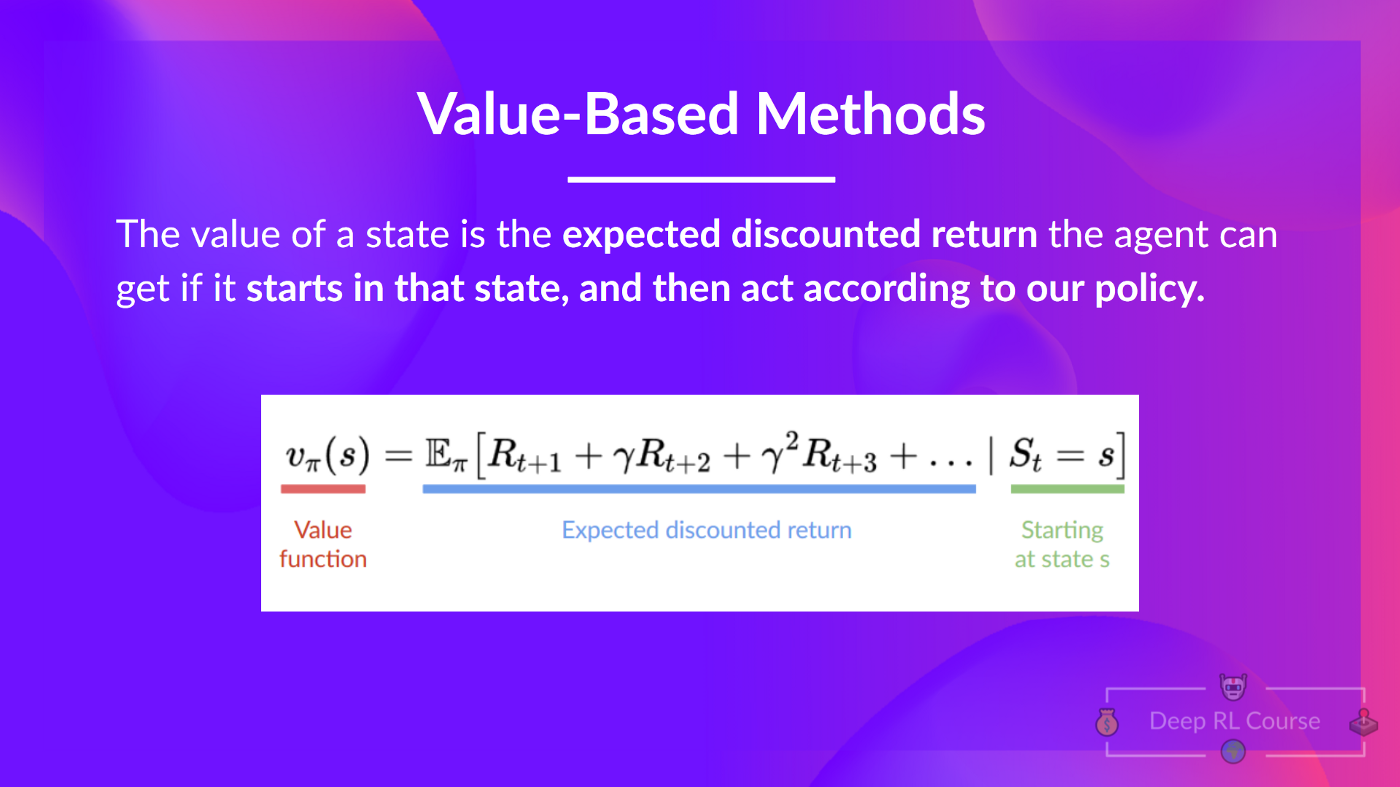
The value of a state is the expected discounted return the agent can get if it starts at that state and then acts according to our policy.
But what does it mean to act according to our policy? After all, we don’t have a policy in value-based methods since we train a value function and not a policy.
To find the optimal policy, we learned about two different methods:
- Policy-based methods: Directly train the policy to select what action to take given a state (or a probability distribution over actions at that state). In this case, we don’t have a value function.
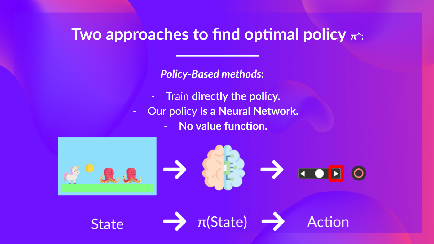
The policy takes a state as input and outputs what action to take at that state (deterministic policy: a policy that output one action given a state, contrary to stochastic policy that output a probability distribution over actions).
And consequently, we don’t define by hand the behavior of our policy; it’s the training that will define it.
- Value-based methods: Indirectly, by training a value function that outputs the value of a state or a state-action pair. Given this value function, our policy will take an action.
Since the policy is not trained/learned, we need to specify its behavior. For instance, if we want a policy that, given the value function, will take actions that always lead to the biggest reward, we’ll create a Greedy Policy.
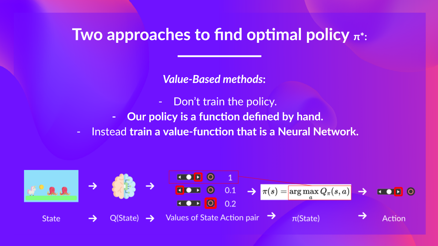 *Given a state, our action-value function (that we train) outputs the value of each action at that state. Then, our pre-defined Greedy Policy selects the action that will yield the highest value given a state or a state action pair. *
Consequently, whatever method you use to solve your problem, you will have a policy. In the case of value-based methods, you don’t train the policy: your policy is just a simple pre-specified function (for instance, the Greedy Policy) that uses the values given by the value-function to select its actions.
So the difference is:
- In policy-based training, the optimal policy (denoted π) is found by training the policy directly.*
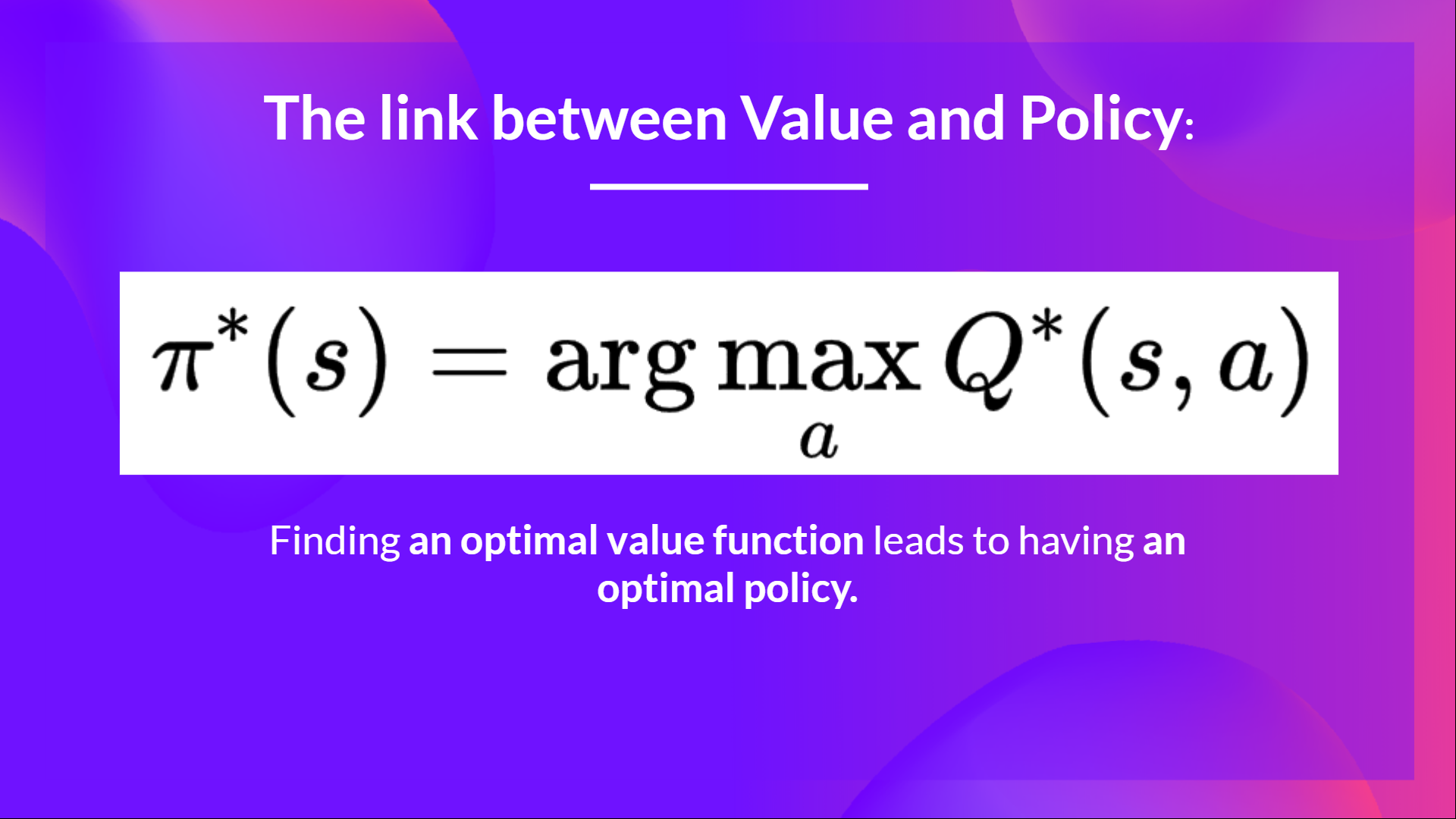
- In value-based training, finding an optimal value function (denoted Q or V, we’ll study the difference below) leads to having an optimal policy.**
In fact, most of the time, in value-based methods, you’ll use an Epsilon-Greedy Policy that handles the exploration/exploitation trade-off; we’ll talk about this when we talk about Q-Learning in the second part of this unit.
argument of the maximum 对于一个函数 f(x) ,argmax 返回的是使 f(x) 最大的那个输入 x ,而不是最大值本身。
As we mentioned above, we have two types of value-based functions:
The state-value function
The action-value function
The value of taking action in states under a policyππ is:
The Bellman Equation , simplify our value Difference Learning
Monte Carlo vs Temporal Difference Learning
蒙特卡洛方法与时间差分学习
Monte Carlo: learning at the end of the episode
Temporal Difference Learning: learning at each step
时序差分学习:每一步进行学习